Stock Price Prediction using SVM and LSTM

 Stock Price Prediction using SVM and LSTM 

• Predicting how the stock market will perform is one of the most difficult things to do. There are so many factors involved in the prediction – physical factors vs. psychological, rational, global markets, Domestic news, finance events, etc. All these aspects combine to make share prices volatile and very difficult to predict with a high degree of accuracy.

• using machine learning we can predict stock more accurately and precisely. In this project, we have worked with historical data about the stock prices of a publicly listed company(Tata Motors). We have implemented a mix of machine learning algorithms to predict the future stock price of the company, starting with algorithms like linear regression, SVM and then move on to advanced techniques like LSTM.

What is the goal of SVM?

Support Vector Machines (SVMs) are mostly used for classification. The goal of an SVM is to define a boundary line between the 2 classes on a graph. This boundary line is called a hyperplane.

How It Works?

Let’s say we have a plot of two label classes as shown in the figure below:

The line fairly separates the classes. This is what SVM essentially does – simple class separation. Now, what is the data was like this:

Here, we don’t have a simple line separating these two classes. So we’ll extend our dimension and introduce a new dimension along the z-axis. We can now separate these two classes:

                              

When we transform this line back to the original plane, it maps to the circular boundary as I’ve shown here:

This is exactly what SVM does! It tries to find a line/hyperplane (in multidimensional space) that separates these two classes. Then it classifies the new point depending on whether it lies on the positive or negative side of the hyperplane depends on the classes to predict.

Why SVR?

With stock data, we are not predicting a class, we are predicting the next value in a series.

Using regression we try to minimize the cost function using something like gradient descent. With SVM we try to draw a hyperplane between 2 different classes. 

So SVR is the combo of the 2, we try to minimize the error within a certain threshold.

The blue line is our hyperplane and the red lines are our boundary lines. We are trying to predict values accurately within a certain threshold. Our goal is to minimize the error and maximize the margin distance. what SVR looks like:

                    

Function to make a prediction using 3 different kernels:

A kernel is a function to map lower-dimensional data into higher dimensional data. We define our kernel to be RBF, poly, and Linear. RBF stands for radial basis function. The equation for RBF is below:

C is the regularization parameter. This is how much you want to avoid misclassifying each training example. For large values of C, the algorithm will choose a smaller-margin hyperplane.

In our case, we choose our C value to be 1e3 which is a large value for C which means our algorithm will choose a smaller-margin hyperplane.

plot the graph:

Here from the past 30day's data, our SVR-RBF model predicts 268.48  and the original value we have is 262.70 which is nearer to the RBF model.

Conclusion:

Here in SVM, there is no concept of memory, and for a large number of data in the stock market with time, there are more other parameters that also affect the stock price like company result, global and local news, or events so that's why for long data we can use LSTM which have the capacity to learn from previous data.

What is LSTM?

LSTM stands for Long Short Term Memory. LSTMs are an advanced version of recurrent neural networks. Recurrent neural networks (RNN) are a special type of neural network. RNNs take the previous output as input. In RNNs the previous output influences the next output.

LSTMs are explicitly designed to avoid the long-term dependency problem. All recurrent neural networks have the form of a chain of repeating modules of neural networks.LSTMs also have this chain-like structure.

Gates inside LSTM cells help the LSTM decide what data is important to be remembered and what data can be forgotten even on long series of data. The type of gates is the forget gate, the input gate, and the output gate. 

The sigmoid layer outputs numbers between zero and one, describing how much of each component should be let through. A value of zero means “let nothing through,” while a value of one means “let everything through!”

Forget gate:

The forget gate takes the previous hidden state from the previous LSTM cell and the current input and multiples them. Values closer to 0 means forget the data, and values closer to 1 means keep this data.

After this is calculated it is passed on to the cell state.

Input gate:

This gate updates the cell state with the new data we want to store in the cell state. The input gate takes the previous hidden state multiplied by the input and passes it through a sigmoid. Values closer to 0 are not important and values closer to 1 are important. Then the previous hidden state is multiplied by the input and passed into an activation function which squishes the values into a range of -1 to 1. Then, the sigmoid output is multiplied by the tan output. The sigmoid output decides what information is important to keep from the tanh output.

Cell State:

The memory of the network. The cell state is the forget gate output * previous cell state + the input gate output * the cell state values passed on from the previous cell. This is to drop certain values that are closer to zero that we want to forget. Then we add the values from the input gate to our cell state value that we want to pass on to the next cell.

Output gate:

The output gate decides what the next hidden state should be. We take the previously hidden state multiply it by the input and pass it into a sigmoid activation function. Then we pass the cell state value into a tan activation function. We then multiply the tan output by the sigmoid output to decide what data the hidden state should carry on to the next LSTM cell.

Model:

Data Set:

Time series problems, values are predicted at interval time T .This model is going to predict the closing stock price of the data based on prices for the past 50 days(50-time step(T) and 1 output). Hence data-set splits into train and label sets. Train sets have past 50 values and Label have corresponding that 51st value which is to be predicted and becomes an input for the next time-step. Similarly time steps are created for whole data-sets. Then data-sets are to be reshape into array as they are in form of lists.

Building the model:

To build the LSTM model by adding layers and dropout layers. were in this model four layers with input layer and output layer(dense layer with one unit)each having no of units and dropout are implemented.Dropout layer is added to avoid over-fitting. Above can be achieved using keras library.

Compile:

Further implemented LSTM model is to be compiled and train, but before training on training data-sets compilation is triggered with a parameter for loss function and optimizer.

Train:

Now next step is to train LSTM model that was build so far by giving parameters train set,label set,number of epochs.Training of model is achieved using Fit() method.

Epochs:

It means, when an entire data-set is passed both forward and backward through the neural network only once, is called one epoch.Each epoch carried out minimum loss in the loss function.

Testing LSTM:

Now after completion of training, the LSTM network is ready for test by making predictions on given test data-sets. As we did with our training data- set similarly test data-sets are also to be shaped to the right format. Prediction is achieved using predict(method) and corresponding graph can be plotted using matplot library.

 

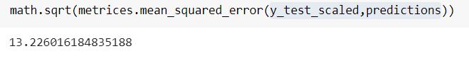
Error calculation:

At last, predicted values and real testing values are compared and then error is calculated. So RMSE(root mean square error) is used for calculate error and percentage error which is re- quired for the accuracy of our model.

Conclusion:

Here We take past 3 years of data in our data set.As we can see in the graph our predicted values are very much similar to the original values from the error calculation we can see that we got around 87% accurate prediction from the above LSTM model. And around 97% accurate prediction using SVM.

As above from SVM and LSTM model here we predict the stock price of tata motors Company which was vary volatile like in 3 years this stock move down to 74 from around 500.and again it move up to 350 in only 3 months from that low. despite we can get very accurate values from that model.

Thank You.